Dedicated to the memory of Piet Hein (1905 - 1996)

A Backtracking Algorithm
Wolfgang Laun
Thales Rail Signalling Solutions GesmbH

Introduction

The algorithm described by Knuth is a "brute force" search using backtracking, which he calls "algorithm X". An efficient implementation is essential for solving non-trivial problems of this kind. The title of Knuth's paper alludes to the proposed solution where the search space is represented as a boolean matrix, sparsely populated with true values, so that it can be represented by a small number of elements being linked to form rows and columns. Progress towards a solution is made by eliminating rows and columns from that matrix; backing up requires eliminated elements to be re-inserted. This algorithm, called DLX, benefits from Knuth's astute observation that unlinked elements may conserve the links to their former neighbours so that re-insertion during a step back in the backtracking procedure does not require an update of the links in the re-inserted element.

Is using "dancing links" also the best solution in Perl? This paper discusses a Perl 5 implementation that represents the search space as a simple two-dimensional array and uses powersets of the index sets for rows and columns to represent the diminishing search space.

Exact Cover Problems

Exact Cover Problems result from a number of mathematical or geometrical puzzles, but they are also closely related to real-world optimization problems.

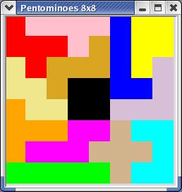
The classic problem (which was attacked with computers as early as 1958) is to find all ways for placing the 12 pentominoes ([5]) on a rectangle of 60 square units or (together with one 2 x 2 square) on an 8 x 8 square. Pentominoes are a special kind of the species polyominoes which are the generalization of dominoes for n = 3, 4, 5,... Thus, a pentomino is a connected shape formed as the union of five identical squares each of which is connected to one or more other squares through a shared edge. The image shows the 12 pentominoes with their customary name.

Several other two-dimensional puzzles have been investigated as well. Knuth applies his algorithm also to hexiamonds and tetrasticks. (See the extensive list of references in [1].)

Chess has inspired the N queens problem, where N queens must be placed on an N x N chess board so that no queen threatens another queen. This can be solved with a classic recursive algorithm ([6]). It can be shown that using algorithm DLX on this problem is significantly faster.

The more recent Sudoku craze has created another application for Knuth's algorithm ([7]).

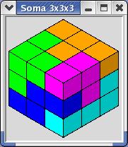
And, finally, there is the Soma cube ([8]), invented by the Danish scientist, mathematician, inventor, author, and poet Piet Hein ([9]). It consists of 6 polycubes of 4 unit cubes, and one v-shaped polycube of 3 units.

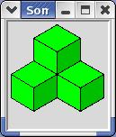
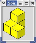
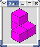
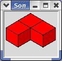
These 7 pieces add up to 27 cubic units, and may be arranged to form a cube and many other shapes. Several programs solving Soma problems have been published (see, for instance [10]), but it is possible that DLX hasn't been applied to this problem before. - The image shows a composite Soma shape ("castle") wherein the individual pieces can be easily recognized.

The Algorithm for the Exact Cover Problem

Defining the Terms of the Problem

We'll refer to the object that is to be covered as the arena, with a subdivision into cells, constituting the "domain set". An object of the candidate set is called tile, and it is defined by its shape, a position within the arena and a set of constraints that block other tiles to be used at the same time. Typical constraints result from the cells to be covered, or from the problem requirement that one shape may only be used once.

Any such problem can be represented as a boolean matrix, where the rows correspond to tiles and the columns correspond to constraints.

The Abstract Algorithm

Given a boolean matrix A, the algorithm (according to [1]) can be formulated as a recursive procedure step

step (A)
   if A is empty then display solution and return
   choose a column c
   for all r so that A[r,c] is true
      include r in the solution set
      for all j so that A[r,j]
         delete column j from A
         for all i so that A[i,j]
            delete row i from A
      call step(A)
      undelete rows and colums
      remove r from the solution set

DLX: Knuth's Algorithm

Pointer Preservation

Knuth's paper is centered around the fact that removing a list node from a doubly linked list without clearing the link field in the node simplifies the re-insertion considerably. It is, of course, absolutely necessary to re-insert nodes in the reverse order of the deletions because any deleted node conserves its state at the time of its deletion.

Selecting the Column

The efficiency of the trial-and-error approach depends considerably on the order of column selections. Selecting a column that leads to a small number of possible row choices is preferable because it means that the search tree has a small fan-out. If the current number of true values per column is available, an efficient selection of the column with the minimum number of true entries is possible.

Implementation in Perl

Doubly linked lists are rare birds in Perl. One author ([2]) states that "actual circular linked lists are quite rare [...] mainly because they're generally not an efficient solution." The imporant word here is generally, and Knuth's algorithm is indeed one place where doubly linked lists apply, even in Perl.

Another Perl book ([3]) discusses linked lists thoroughly. Doubly linked lists are implemented with objects based on hashes. As we are going to need a very efficient implementation, we'll avoid hashes and object oriented techniques. Below is a (somewhat shortened) listing of the Perl module Node, where the node variable (implemented as a simple array) provides the link fields for two doubly linked lists, one linking nodes within a row (using the L and R fields) and within a column (U and D).

package Node;

use constant iL => 0;
use constant iR => 1;
use constant iU => 2;
use constant iD => 3;
use constant iR => 4;
use constant iC => 5;

sub new {
    my( $col, $row ) = @_;
    my @node = ( 0, 0, 0, 0, $row, $col );
    $node[iL] =
    $node[iR] =
    $node[iU] =
    $node[iD] = \@node;
}

sub L { shift->[iL]; }
sub R { shift->[iR]; }
sub U { shift->[iU]; }
sub D { shift->[iD]; }
sub C { shift->[iC]; }
sub R { shift->[iR]; }

sub unlinkLR {
    my $self = $_[0];
    $self->[iL]->[iR] = $self->[iR];
    $self->[iR]->[iL] = $self->[iL];
}

sub unlinkUD { ... }

sub insertLR {
    my( $self, $node ) = @_;
    $node->[iR] = $self->[iL]->[iR];
    $node->[iL] = $self->[iL];
    $self->[iL]->[iR] = $node;
    $self->[iL] = $node;
}

sub insertUD { ... }

sub restoreLR {
    my( $self ) = @_;
    $self->[iL]->[iR] = $self;
    $self->[iR]->[iL] = $self;
}

sub restoreUD { ... }

The column "objects" can be represented as simple extensions to the Node data structure. Field S stores the count of ones in the column, and field N contains a column identification. In addition to the functions retrieving the field values, there are only functions for incrementing and decrementing the count field.

package Column;

use Node;

use constant iS => 6;
use constant iN => 7;

sub new {
    my( $root, $name ) = @_;
    my $obj = Node::new( $root );
    push( @$obj, 0, $name );
    return $obj;
}

sub S { shift->[iS]; }
sub N { shift->[iN]; }

sub incS { shift->[iS]++; }
sub decS { shift->[iS]--; }

Implementation Alternatives

Package Node is quite close to an object oriented implementation. An object-oriented implementation requires a constructor returning a blessed reference, which could be an array or a hash reference. Using an array, only new would have to be rewritten as

sub new {
    my( $class, $row, $col ) = @_;
    my @node = ( 0, 0, 0, 0, $row, $col );
    $node[iL] =
    $node[iR] =
    $node[iU] =
    $node[iD] = \@node;
    return bless( \@node, $class );
}

sub new {
    my( $class, $row, $col ) = @_;
    my %node = ( iL => 0, iR => 0, iU => 0, iD => 0,
                 iT => $row, iC => $col );
    $node{iL} =
    $node{iR} =
    $node{iU} =
    $node{iD} = \%node;
    return bless( \%node, $class );
}

It's now possible to benchmark all possibilities, comparing an unlink/restore and an unlink/insert operation for both doubly linked lists.

Technique	restoreXY	insertXY
not OO	6.68	8.53
OO - array	7.03	8.91
OO - hash	7.81	9.81

1. Object-orientedness causes a small penalty which is tolerable except where very high performance is required.
2. Implementing objects based on arrays is significantly faster than using hashes.
3. But, above all, look out for the better algorithm before you complain about missing implementation techniques.

The Core: DLX::solve

sub solve {
    my $column;

    # Do we have another solution?
    if( ( $column = R( $Root ) ) == $Root ){
	$SolCount++;
	my $elapsed = tv_interval( $StartTime, [ gettimeofday() ] );
        my @sol = map( $Row2Tile[T( $_ )], @Solution );
        $Arena->showSolution( $SolCount, $elapsed, @sol );
        return;
    }

    # choose another column: minimum "true" count
    my $size = S( $column );
    for( my $iCol = $column; $iCol != $Root; $iCol = R( $iCol ) ){
        my $ics;
	if( ( $ics = S( $iCol ) ) < $size ){
            $column = $iCol;
            $size = $ics;
	}
    }

    # cover selected column
    cover( $column );

    # loop over the rows
    for( my $iRow = D( $column ); $iRow != $column; $iRow = D( $iRow ) ){
        push( @Solution, $iRow );
        for( my $jCol = R( $iRow ); $jCol != $iRow; $jCol = R( $jCol ) ){
            cover( C( $jCol ) );
	}
        solve();
        $iRow = pop( @Solution );
        $column = C( $iRow );
        for( my $jCol = L( $iRow ); $jCol != $iRow; $jCol = L( $jCol ) ){
            uncover( C( $jCol ) );
	}
    }
    uncover( $column );
}

sub cover {
    my $c = shift;
    # remove it from header list
    unlinkLR( $c );

    # remove all rows in the column's own list
    for( my $iRow = D( $c ); $iRow != $c; $iRow = D( $iRow ) ){
        for( my $jCol = R( $iRow ); $jCol != $iRow; $jCol = R ($jCol ) ){
            unlinkUD( $jCol );
            decS( C( $jCol ) );
	}
    }
}

sub uncover {
    my $c = shift;
    # restore unlinked elements
    for( my $iRow = U( $c ); $iRow != $c; $iRow = U( $iRow ) ){
        for( my $jCol = L( $iRow ); $jCol != $iRow; $jCol = L( $jCol ) ){
	    incS( C( $jCol ) );
            restoreUD( $jCol );
	}
    }
    restoreLR( $c );
}

Modifications

Detecting Solutions

Algorithm DLX has found another solution as soon as the matrix is empty. This requires that the matrix is reduced once more after the final tile has been placed. If we assume that it is not necessary to demonstrate that all cells of the arena have indeed been covered, we may claim another solution as soon as the count of solutions in the solution stack has reached the expected number of tiles or some similar test.

Reducing the Size of the Matrix

One of the major factors influencing the efficiency of the search is the size of the matrix. Avoiding columns isn't possible but there may very well be criteria that eliminate rows from any solution. One row is required for all tiles in all feasible positions, so the question is whether it can be decided that a feasible position doe not occur in a solution. Obviously this depends on the properties of the problem.

Impossible Pentomino Positions

With some arena shapes there are feasible pentomino positions that cannot occur in any solution. In the 20 x 3 rectangle, the "x" pentomino cannot be placed at the extreme ends because this would cut off two squares of area one. Also, it cannot be placed two columns from either small side as this would cut off areas of 8 square units. In general, we can formulate the condition that all adjoining simply connected free areas must have an area that is an integer multiple of 5.

The implementation is fairly simple. After placing a pentomino into an otherwise free arena, visit all of its squares and "flood fill" all free neighbours, counting the flooded squares. If any such fill operation returns a cell count that is not a multiple of 5, the position may be discarded.

Certain patterns place severe restrictions on the "mobility" of the pentominoes within the arena. The diamond shape shown below is one of these patterns.

If we color the cells of this shape like a chess board, we see that the ratio between the colors is 36:24. Eleven of the individual pentominoes can be colored with a ratio of 3:2, and the "X" pentomino has 4:1. To achieve the shape's overall ratio, all pentominos must be placed so that they favour the same board field colour. This would result in a considerable reduction of matrix rows and, thus, computing time. (In fact, this pattern has no solution at all.)

Impossible Polycube Positions

Other reductions may be possible for certain arenas. The cube, for instance, requires that the "T" shape pentomino is positioned along one of the edges. (An elegant proof of this can be found in [4].)

Exploiting Symmetry

Symmetric arenas produce symmetric solutions. It is possible to avoid solutions which are reflections or rotations of a principal solution by selecting one piece and limit its position suitably to a section of the arena. This will also reduce computing times accordingly.

Choice of Column

Investigating Powersets

The Idea

Eliminating some elements from a set and returning them again: Such operations are frequently implemented using sets, which can be efficiently mapped to bit vectors. If we accept the potentially quite hefty (O(10⁶) elements) memory requirement of the full matrix A, we can represent present rows and present columns by a set of row and column indices, respectively. Keeping both rows and columns of matrix A as bit sets enables us to manipulate sets of row and column indices quickly, without the need to access matrix elements individually so that covering and uncovering may be implemented as set operations. This means that we can get rid of several explicit loops.

Sets can be implement in Perl 5 by exploiting the builtin function vec which operates on byte strings as if they were packed arrays of bit fields with a size equal to 1 (or any other power of 2 up to 32 or 64). Also, such byte strings can be operands of the bitwise operators "|", "&", "^", and "~". Such an operation will execute its loop "inside", in C code, which is considerably faster than at Perl level.

Package Bitset

package Bitset;

sub new($){
    my( $size ) = @_;    
    return "\0" x (($size+7)/8);
}

sub and(\$$){
    ${$_[0]} &= $_[1];
}

sub andNot(\$$){
    ${$_[0]} &= ~ $_[1];
}

sub or(\$$){
    ${$_[0]} |= $_[1];
}

sub get(\$$){
    return vec( ${$_[0]}, $_[1], 1 );
}

sub set(\$$){
    vec( ${$_[0]}, $_[1], 1 ) = 1;
}

sub clear(\$$){
    vec( ${$_[0]}, $_[1], 1 ) = 0;
}

sub size($) {
    return 8*length( $_[0] );
}

# nextBit( bitstr, offset )
#
sub nextBit(\$$){
    my $max = 8*length( $$_[0] );
    for( my $iPos = $_[1]; $iPos < $max; $iPos++ ){
	if( vec( $$_[0], $iPos, 1 ) ){
	    return $iPos;
	}
    }
    return -1;
}

my @bits = (
[  ],
[ 0 ],
[ 1 ],
[ 0, 1 ],
[ 2 ],
[ 0, 2 ],
[ 1, 2 ],
[ 0, 1, 2 ],
...
[ 2, 3, 4, 5, 6, 7 ],
[ 0, 2, 3, 4, 5, 6, 7 ],
[ 1, 2, 3, 4, 5, 6, 7 ],
[ 0, 1, 2, 3, 4, 5, 6, 7 ],
    );

sub getIndices {
    my $ic = 0;
    map { my $c = $ic++; map { 8*$c+$_ } @{$bits[$_]}; }
          unpack( 'C' . length($_[0]), $_[0] );
}

sub card {
    return unpack( '%32b*', $_[0] );
}

The Core: BSX::solve

sub solve {

    if( $ColSet eq $EmptyColSet ){
	$SolCount++;
	my $elapsed = tv_interval( $StartTime, [ gettimeofday() ] );
	$Arena->showSolution( $SolCount, $elapsed, @Solution );
        return;
    }

    my $column;
    my $size = 0x7fffffff;
    for my $iCol ( getIndices( $ColSet ) ){
	if( $OneCount[$iCol] < $size ){
            $size = $OneCount[$iCol];
            $column = $iCol;
	}
    }

    # for a row r so that A[r,c] is set
    #
    for my $iRow ( getIndices( $RowSet ) ){
	my $matRow = $A[$iRow];
	if( $matRow->[$column] ){

	    # include row in partial solution
	    push( @Solution, $Row2Tile[$iRow] );

            # save current state of the matrix (rows and columns)
	    my $savRowSet = $RowSet;
	    my $savColSet = $ColSet;

	    # delete columns and rows

            # all columns where the current row is true
            my $redColSet = $BitsInRow[$iRow];
	    Bitset::and( $redColSet, $ColSet );

            # all rows where there is true in any of the deleted columns
            my $redRowSet = $EmptyRowSet;
	    for my $iCol ( getIndices( $redColSet ) ){
                Bitset::or( $redRowSet, $BitsInCol[$iCol] );
	    }
	    Bitset::and( $redRowSet, $RowSet );
            Bitset::andNot( $RowSet, $redRowSet );

            # delete the columns
            Bitset::andNot( $ColSet, $redColSet );

            solve();

            $ColSet = $savColSet;
            $RowSet = $savRowSet;
	    pop( @Solution );
	}
    }
}

And the Winner Is...

Test Programs

Pentominoes

The packages PentominoBoard, Square, Position2D, PentominoFactory and ArenaDisplay implement the essential framework required for setting up the abstract Exact Cover Problem handled by DLX or BSX. The display function is implemented using Perl::Tk, resulting in a pretty show while the algorithm plods through the solutions.

The arena is implemented by the class PentominoBoard. After setting (maximum) width and height, individual cells can be removed from the arena. The class PentominoFactory cooperates with a board object, to create all tiles. Each tile must pass the flood fill test before another row of the matrix is created from it. (This is helpful with the narrow rectangles 3x20 and 4x15.)

The Soma Cube and Other Shapes

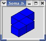
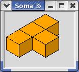
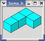
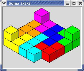
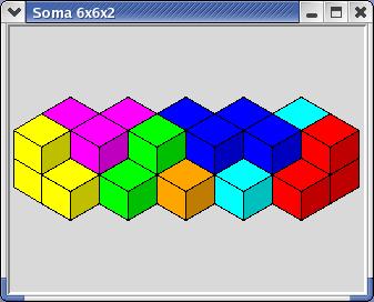
The packages SomaSpace, Cube, Position3D, SomaFactory and SpaceDisplay provide the setup for a three dimensional arena and the pieces of the Soma cube as tiles. The test program (somatest.pl) provides a selection of popular Soma figures. (See [11] for a comprehensive collection.) Here is one solution for the cube:

The class SomaSpace provides functions for defining a three dimensional arena, and for removing and adding cells so that even fissured shapes can be constructed. Flood filling is employed here as well, although only some figures benefit from it.

Benchmarks

The table below shows the execution times for several Soma shapes. The column titled "Matrix" shows the dimensions of the matrix A.

Shape	Matrix	Solutions	DLX	BSX
Cube	688x34	11520	255.62	232.71
Tower	427x34	1520	19.00	7.24
Stairs	328x34	328	16.25	5.33
Steamer	264x34	304	2.09	0.91
Well	307x34	294	3.11	0.69

It is obvious that execution times should depend on the size of the matrix, mainly upon the number of rows. Knowing all the implementation details, it is fairly easy to interpret the other aspects of these results.

• Algorithm DLX is not slowed down significantly by an increasing number of matrix rows, because the number of true elements within a column does not increase proportionally.
• Algorithm BSX is faster for smaller row counts. This is due to the absence of almost all loops.
• The old wisdom that there is no such thing as a single "best algorithm" has been confirmed once more. (Notice that both the Pentomino and the Soma cube problems can be solved faster with individually designed programs.)

The results for the Pentomino solver are somewhat disappointing, but no surprise, since the row counts increase significantly as the rectangles become wider.

Board	Matrix	Solutions	DLX	BSX
3x20	728x72	8	8.83	12.73
4x15	1450x72	1472	1384.00	< ∞
64-3,3	1432x72	1520	719.28	< ∞

All times were obtained on an Intel Pentium 600MHz processor.

Conclusion

Even though NP-complete problems are renowned for their considerable hunger for CPU time, Perl has enabled us to investigate two algorithms for the Exact Cover Problem, and to create a pretty set of demonstrations.

Perl's flexibility - the famous TIMTOWTDI - lets you use object oriented techniques where you gain from code reuse and abstract algorithms, while you can still use the procedural style where efficiency is paramount.

Therefore, I think it is more than justified to say that the winner is - the Perl Programmer.

References

[1] Donald E. Knuth "Dancing Links," http://www-cs-faculty.stanford.edu/~knuth/papers/dancing-color.ps.gz

[2] Damian Conway, Perl Best Practices, O'Reilly, 2005

[3] Jon Orwant, Jarkko Hietaniemi, John Macdonald, Algorithms with Perl, O'Reilly, 1999

[4] Erhard Quaisser, Diskrete Geometrie, (Heidelberg: Spektrum Akademischer Verlag, 1994)

[5] Martin Gardner, The Scientific American Book of Mathematical Puzzles and Diversions (New York: Simon & Schuster, 1959)

[6] Ole-Johan Dahl, Edsger W. Dijkstra, C.A.R. Hoare, Structured Programming (London: Academic Press, 1972)

[7] Daniel Seiler, "Dancing Sudoku," http://dancingsudoku.sourceforge.net

[8] Martin Gardner, The Second Scientific American Book of Mathematical Puzzles and Diversions (New York: Simon & Schuster, 1961)

[9] Wikipedia, "Piet Hein (Denmark)," http://en.wikipedia.org/wiki/Piet_Hein_(Denmark)

[10] Bruce Cropley, "PCSolve," http://www.fam-bundgaard.dk/SOMA/NEWS/N031026.HTM

[11] Thorleif's SOMA page http://www.fam-bundgaard.dk/SOMA/FIGURES/FIGURES.HTM