AnTherm (Thermal Bridges)

AnTherm (Analysis of Thermal behavior of Building Construction Heat Bridges) is a powerful package of programs used for heat flow calculation in building construction elements - the thermal bridges.

The basic knowledge on thermal bridges and heat flow/transportation is provided in book "Wärmebrücken". It also provides the description of Conductance Matrix (Leitwert Matirx).

Furthermore, the program allows calculation of:

2D and 3D - two and three dimensional heat flow and vapour diffusion
computing of Conductance Matrix Values (Leitwerte) and Psi-Values
stationary (and soon instationary (periodic)) heat flow
dew point on the surface and inside of the construction

AnTherm is a powerful program package for the calculation of temperature distributions and heat flows in building structures - particularly such with thermal bridges. For the technically qualified designer, AnTherm is a reliable, indispensable tool in meeting the demands of the current European standards (EN) for evaluating thermal performance thoroughly and precisely.

Interested? Contact me for more.

Please visit http://antherm.kornicki.com site which is fully dedicated to that program.

AnTherm analyses temperature conditions in building components in which heat flows not just in one direction, but in two- and three-dimensional patterns. This is of critical interest when evaluating the thermal performance - an important design criteria - of so-called thermal bridges, that is, regions of a building construction through which local peaks of heat loss can cause surface temperatures to drop below the dewpoint. Thermal bridges are characterised by multi-dimensional heat flow, and therefore by the fact that they cannot be adequately approximated by the one-dimensional models of calculation typically used in norms and standards for the thermal performance of buildings (U-values).

The method of analysis most commonly practiced today when evaluating the thermal performance of building spaces, components, and assemblies is based on a simple, one-dimensional, constant flow model of heat conduction (i.e. the assumption of parallel heat flow for the calculation of U-values and areas). Such an assumption often leads not only to disappointing results in the thermal performance of realised construction projects, but also to costly consequences due to unforeseeably high energy consumption for heating, as well as damage caused by surface condensation of moisture.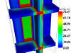

These potentially negative consequences of over-simplification, inherent to the assumption of one-dimensionality, are becoming increasingly critical in today's trend towards highly insulated building structures. If the effects of thermal bridges are neglected, drastic errors in estimating heating requirements are bound to result, particularly when assessing energy efficient buildings. Multi-dimensional (i.e. two- and three-dimensional) evaluations of thermally critical regions within a building assembly during early design phases can provide valuable preliminary information to support the decision-making process, thus leading to considerably more reliable design results.

Surface moisture due to condensation (typically occurring in such regions as floor-wall connections, window installations, etc.) as well as mould growth in humid environments can also be effectively prevented by means of multi-dimensional evaluation during planning and detail design.

European Standards (EN) pertaining to such aspects of thermal performance of building constructions are already available . The ramifications of the adoption of these European Standards is apparent: they describe the substance of new tasks for designers, manufacturers, and builders, as well as their significance for quality control in the field of energy conservation.

The purpose of the standard EN "Thermal Bridges - Calculation of Surface Temperatures and Heat flows" is explicitly stated as:

the calculation of minimum surface temperature in order to assess the risk of surface condensation and
the calculation of heat flows (for the constant flow case) in order to predict overall heat loss from a building.

Furthermore, "high precision" methods of calculation are demanded, whereby precision criteria which must be satisfied by the method chosen are defined in the standard.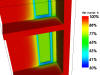

According to EN "Building Components or Building Elements - Calculation of Thermal Transmittance", calculation of heat transfer coefficients of parallel plane surface building components shall be performed based, of course, on one-dimensional models. For such components, composed of surface parallel layers of thermally homogeneous or non-homogeneous materials, a well-known method of estimation (ISO-method) can be implemented in order to obtain a design thermal resistance - assuming the maximum relative error remains "negligible".

For all other heat flow patterns, i.e. for all cases of more than one dimension, in particular in the presence of thermal bridges, the standard EN "Thermal Bridges" requires the implementation of numerical methods of evaluation.

The program AnTherm meets the demands of the European Standards with respect to input data and - more importantly - output data requirements (evaluation results).

With respect to input data, AnTherm

facilitates the generation of geometrical models by supporting a graphic input display of building structures, as well as by providing an entirely independent, fully automatic method of fine subdivision (which can also be influenced by the user through manual manipulation of parameters).
delivers complete input model documentation (geometry of material elements, thermal design values of materials, spaces, heat sources...) upon request.
allows the precision of numerical solutions to be influenced and controlled by the user (definition of calculation parameters).

Evaluation results yielded by AnTherm include

generally applicable results in the form of g-values and conductance matrices. These conform to the temperature weighting factors and "thermal coupling coefficients" defined in the European Standards, including the required information on calculation precision.
specific results, applicable to particular air temperature conditions in spaces thermally coupled by the building components analysed, in the form of surface temperature minima and maxima as well as respective dewpoints.
graphic plots and prints of isotherms, surface temperatures or temperatures along an edge (2- or 3-dim. models), as well as heat flow diagrams (not limited to 2-dim. models only, but also in 3D).

Furthermore, fully automatic execution of calculation with AnTherm is given even in the event of poorly conditioned calculation cases. The maximum quantity of balancable cells is nearly unlimited (many millions), thus making the thorough analysis of large, three-dimensional models feasible. Complex cases are given, for example, by

components or spaces in contact with ground.
entire spatial envelopes or groups of spaces.
detailed modelling of complicated assemblies (window frame and installation details, steel structures, etc.).

The thermal performance of building assemblies with overall dimensions of up to app. 100 m can be simulated with AnTherm. Limitations to the scope of evaluation depend on the PC hardware implemented.

Interested? Contact me for more.

System Requirements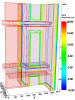

The computer hardware necessary for running the program package AnTherm successfully depends on the nature (and complexity) of the constructions to be analysed as well as on the quality of results precision sought by the user. Both factors affect the number of equations which must be solved in the course of calculation. This number is limited primarily by the amount of memory available. Therefore, if an emphasis on three-dimensional applications can be expected, a more powerful configuration than the minimum described here is advisable.

Hardware:

PC compatible with Windows XP or Vista
512 MByte memory (minimum, 2048 MByte optimal)
200 MByte free disk space (for installation only)
Screen resolution of 1024x768 (minimum, 1280x1024 optimal)
Supporting 3D OpenGL graphics (minimum, optimum with 3D accelerated graphics board)
B/W Printer A4 (minimum, color printer optimal)

Software:

MS Windows Windows XP or newer (XP optimal)
Microsoft® .NET 1.1 Runtime installed (can be freely installed as an option directly from Microsoft)
A License to use the program AnTherm

As already mentioned, the maximum number of cells (model size) which can be calculated depends primarily on the memory capacity of the computer used. The highest memory load is expected during 3D graphics visualisation within the final evaluation process.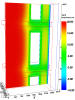

The computation time to be expected in calculating a particular model depends on the speed (frequency) and grade of the processor(s) used. With a Pentium 4 at 2 GHz processor, for example, the two-dimensional model described in the Tutorial of AnTherm (about of 1500 cells) was calculated in less than 5 seconds. The three-dimensional, extended model of the tutorial object (about of 70000 cells) required 12 seconds from calculation branch begin to return to the Main Menu. Same model calculated at higher cell density (i.e. at finer grid parameters) resulting in about 330.000 cells needed 80 seconds to initially solve.

Interested? Contact me for more.

Primary Concepts

The various terms and theoretical concepts, which form the basis for understanding the AnTherm application, are presented and defined briefly in the following sections. For a more thorough explanation of the theoretical background, please refer to the book "Wärmebrücken".

Environmental Factors

When analysing the thermal performance of building components, two different types of information are sought: thermal transmission and surface temperatures.

The first type entails evaluating the heat transfer characteristics of a building assembly, i.e. the form and quantity of heat losses and gains, in order to ultimately obtain

a reliable estimation of heating and cooling loads (costs),
acceptable heat flow rates, as well as * energy conserving design alternatives.

as well as

energy conserving design alternatives.

Based on the heat transfer characteristics of a construction, the expected temperatures along interior surfaces must be evaluated in order to predict (and avoid) areas of potential moisture condensation. Beyond preventing damage to building materials caused by mould growth, adequate surface temperatures are also a relevant factor in the thermal comfort of an interior environment.

Thermal Transmission

Energy in the form of heat in building constructions is generally transmitted by a combination of conduction, convection, and radiation. When considering heat transfer within and through solid (homogeneous or non-homogeneous) building materials, heat conduction is the primary transmission factor; the effects of convection and radiation are typically negligible.

heat conduction

Conduction through homogeneous planar building components (i.e. composed of one or more layers of material with parallel surface planes) occurs in a single direction: normal to the component surface. This is referred to as one-dimensional heat flow, and is characterised by a constant surface temperature over the entire surface plane.

Such idealised conditions can, of course, only be assumed in limited regions of an actual building structure. Geometries of non-planar components (construction joints, floor-wall connections, balconies, etc.) give rise to heat flow patterns of more than one direction, that is, to two- or three-dimensional heat flow.

thermal bridge

Regions or elements of a building construction characterised by multi-dimensional heat flow patterns are called thermal bridges. In contrast to regions of one-dimensional heat flow, thermal bridges are typically associated with local peaks of heat loss, which correspond to characteristic drops in the interior surface temperature.

Conductance

An exact description of the thermal behaviour of a building assembly would by nature be non-linear, and thus very complicated to evaluate. Fortunately, for most construction situations of interest, it is possible to drastically reduce the complexity of the physical model without sacrificing any appreciable accuracy.

A linear description of thermal transmission involving an entire building can be introduced by

assuming that the temperature of each environment (space) associated with the building is unique, i.e. independent of position, and
forfeiting an exact treatment of radiation exchange within the spaces in favour of an approximation of this factor through adjusted surface transfer coefficients.

thermal conductance	In light of this simplified physical model, it can be stated that the amount of heat which flows from one space to another, Q, is proportional to the temperature difference between the two environments under consideration (i and j). The factor of proportionality is a conductance , L_ij, and linearly defined by Q = L_ij • ( T_i − T_j)
conductance matrix	The analogy of an electrical circuit can be extended to model a building structure more generally as a set of environments thermally connected through a resistance, i.e. the heat-conducting material elements. A complete description of the thermal relationships in a particular structure is given by a conductance matrix of values for all thermal connections, i • j, between the spaces of the model. The conductance matrix defines the heat transfer characteristics of a given model based solely on the geometry and materials (thermal properties) of the resistance, that is, independently of temperature conditions in adjacent spaces. This matrix is symmetrical.
thermal transmittance	The area-related term "thermal transmittance" (U-value in Wm^-2K^-1) commonly used in standards to date essentially describes the same conductance as the reciprocal of the sum of resistances of a planar component, that is, resistances in "series": 1/U = 1/α_i + R + 1/α_e whereby α_i and α_e are the surface transfer coefficients of the interior and exterior environments, and R represents the sum of material resistances of j constituent component layers. The resistance of an individual homogeneous (isotropic) layer is directly proportional to layer thickness, d, and indirectly proportional to the material conductivity, λ: R_j = d/λ However, this simple formula applies only to the planar regions of a building assembly in which strictly one-dimensional heat flow can be reasonably assumed.
length-related conductance	A further type of special situation is given where two-dimensional heat flow patterns are to be expected. Such a region is a stretch of the building assembly which can be evaluated with respect to a two-dimensional section - under the assumption that no heat flow occurs normal to the section plane. In this case, a length-related conductance, L^2D [Wm^-1K^-1], must be calculated for the applicable region. The most general case, of course, is that of three-dimensional heat flow. For the regions of a construction in which no directional assumptions can be made about local heat flow patterns, only the evaluation of the (3D) conductance, L^3D [WK^-1], provides a reliable indicator of the thermal behaviour.
total conductance	Due to the linearity of conductances, an entire building can be modelled as a sum of parts, with each part evaluated according to the applicable geometric conditions. Of course, the summation of conductances is only applicable if the temperature difference is the same through all model parts (e.g. one interior and one exerior temperature valid for the whole building). The model is sub-divided by introducing theoretical cut-off planes, which must be located such that any potential heat flow through these planes can be considered negligible. The total thermal conductance of a building thus modelled can be written as whereby l_j is the length over which the two-dimensional conductance, L^2D, is valid for part j, and A_k is the area of validity for U_k. This reliable and flexible approach to analysing the thermal performance of buildings is referred to in the European Standards as the direct method. It requires the implementation of a suitable computer program for attaining two- and three-dimensional conductance results with the necessary precision The program AnTherm makes use of the linear nature of the heat conduction model by first determining a generally applicable calculation model: a characteristic set of temperature-independent base solutions (see the next section on Method of Analysis).

Surface Temperatures

Once the base solutions describing a particular model have been established, temperature (boundary) conditions can be applied in the adjacent environments in order to predict a specific temperature distribution in the building component.

dewpoint

Here the temperature along the component surface - where condensation is most likely to occur - is of particular interest. Humidity exceeding the saturation level of an environment, i.e. the dewpoint [%], leads to condensation. This value is directly linked to the temperature at any given location under.

temperature extremes

Therefore surface points at which a temperature minimum can be expected to occur must be localised in the model and explicitly evaluated with respect to specified conditions:

boundary conditions - air temperatures [°C]
position of coldest surface point (x, y, and z coordinates)
temperature of the surface at this point [°C]
associated dewpoint [%]

Note: Temperature maxima, i.e. warmest surface points, are primarily of interest when assessing the factor of thermal comfort in constructions which include heat sources. For example, situations in which electrical heating could be implemented (as floor heating, or as a measure against condensation) may be evaluated comparatively to determine if the power output needed could lead to uncomfortably high surface temperatures.

Building elements which absorb and re-emanate solar gain can also be effectively approximated as heat sources and thus evaluated in order to assess constructions critically affected by solar radiation.

Weighting Factors

The air temperatures set in the spaces adjacent to a building component all contribute to the temperature distribution resulting within the component. Therefore, the specific temperature, T, at any given point in a model can also be described as the result of all the space temperatures, T₀ through T_n, weighted for the specific position and summed:

T = g₀•T₀ + g₁•T₁ + … g_n•T_n

g-values

The set of weighting factors, g₀ through g_n, must be determined for each point of the model to be considered more closely. These so-called g-values are normalised such that their sum is equal to one.

If all the interior spaces are set at the same temperature (T_i for T₁ through T_n), and T₀ is defined as the exterior temperature (T_e), then the equation above can be simplified to

T = g₀•T_e + (1 − g₀)•T_i

and re-written as

T = T_i− g₀• ( T_i − T_e )

In this case, g₀ represents a generalised version of the f-value familiar from the evaluation of surface temperatures for one-dimensional heat flow (based on U-values). Contrary to a conventional f-value, which applies to the entire interior surface plane, the g-value above is only valid for a specific point of a thermal bridge.

Once g-values have been characterised for the coldest points of all interior surfaces, however, the temperatures resulting at these points can be evaluated as simply as with the one-dimensional method.

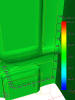
Graphic Representation of Heat Flow

Since the heat flow pattern of a thermal bridge is characteristically more complex than the single-direction flow through a planar component, graphic illustrations of bridge flow patterns can provide critical information at a glance.

heat flow diagram

One method of visualising heat flow is to delineate the direction of flow (vector) through the building component with lines drawn at prescribed intervals. The area bounded by two lines in the diagram represents a heat quantity defined by the interval (e.g. given 10 intervals, the heat flow between two lines corresponds to 10% of the total heat flow in one direction through the surface of a given space). The denser the lines in a region of such a diagram, the more heat flows through this region. Thus local peaks of heat loss (and predictably cold surface points) are easily discernible.

Due to the two-dimensionality of graphic illustrations, however, three-dimensional heat flow patterns cannot be meaningfully rendered with such a diagram. Therefore the three-dimensional rendering provides one streamline through the arbitrary chosen point.

isotherms

The second common method of heat flow representation is to render the temperature distribution in a component with isotherms, i.e. by delineating lines of the same temperature at defined intervals. Isotherms lie normal to the direction of heat flow, thus providing an "inverted" rendering of the heat flow pattern (denser isotherms correspond to regions of increased heat flow).

Since isotherms represent a two-dimensional section through a temperature distribution rather than vectors directly, the isotherm method is also suited for (partial) rendering of three-dimensional heat flow situations.

Method of Analysis

Heat flow in a building construction, as well as the subsequent temperature distribution, can be described mathematically by differential equations. Most importantly, these equations are linear and homogenous by nature.

base solutions

This means that one set of solutions, calculated for a specific set of conditions, can be "re-used" as the basis for solutions under differing conditions by superposition, i.e. by linear combination of selected base solutions. More specifically, base solutions are calculated under the assumption of a "basic" set of boundary conditions: with an air temperature of 1 in the selected space, and 0 in all others.

Thus the temperature distribution, a function of the three spatial coordinates, can ultimately be written in the simple form of a sum of temperature values. The individual temperatures are the result of the actual boundary conditions (air temperatures in the given spaces from 0 to m) weighted by dimensionless base solutions:

In other words, base solutions are effectively a generalised form of weighting factors (g-values) - a function of position for a given space, j: g_j(x,y,z).

The calculation approach in the program AnTherm uses this circumstance to minimise over-all evaluation time. One set of base solutions need be calculated only once to characterise a given model, which can subsequently be considered under varying conditions without repeating the time-consuming computation necessary to solve the primary set of differential equations.

Computation time is further reduced by utilising the weighting function character of base solutions (normalised such that their sum must equal 1). Hence, if n cases have been selected, only n-1 solutions need to actually be calculated. The n-th base solution is then very simply derived as a difference of the sum to 1, that is, by a separate stage of superposition.

Calculation Model

Using the concept of a conductance, L_ij (between the spaces i and j), the heat which flows out of space i is a sum depending on the temperatures of space i and of all other spaces, j:

Since L_ij can be proven to be symmetrical (= L_ji), this equation corresponds formally to Kirchhoff's law of electrical networks. The analogy that this allows is quite significant: the spaces of a building construction (model) can be thought of as nodes in a heat conducting network.

equation model

Thus the heat conduction model, otherwise only describable with partial differential equations, can be mathematically defined as a relatively simple, linear system of equations with a given conductance matrix. Furthermore, only the thermal coupling between spaces which interchange heat directly through the building component ("neighbouring spaces") is of practical effect; coupling between indirectly connected spaces is generally negligible.

conditions

As the equation above shows, in addition to the appropriate value in the conductance matrix, either air temperature or heating load must be defined for each space of the model (evaluation conditions) in order to attain a complete description of a particular heat flow situation.

Numerical Solution

The calculation method of finite differences used by AnTherm is based on the sub-division of the heat conducting continuum into an orthogonal cell structure. Each cell of this calculation geometry is treated as a node of the thermal network, and is typically connected with six other such nodes. The conductance of each connection depends on cell size and thermal conductivity of the material "filling" the individual cells. Therefore, the cell structure must be defined such that each cell can be assigned a single, homogeneous material.

calculation geometry	The calculation geometry is obtained by means of gridding the construction geometry of the model to be evaluated. A concrete grid is generated by dividing the model with a series of grid planes along material boundaries and at additional intervals (their number and distance depends on the precision of analysis required) parallel to the coordinate axes. Once the network data has been sufficiently defined for calculation, the program sets up an appropriate linear system of equations automatically. This equation system then needs to be solved numerically with an iterative method.
relaxation factor	The convergence process of the relaxation method used by AnTherm is entirely dependant on the value of the relaxation factor ω. Initially this factor is defined only within a given range: 1 ≤ ω < 2 The "optimal" ω-value is defined as the constant value of ω which leads to the most expedient convergence of the calculation method. This value differs from case to case and is initially unknown. Once the system of equations describing the model has been determined, the first stage of calculation is therefore an analysis of this system, followed by an iterative calculation to approximate a preliminary "optimal" *-value, ω₀. This stage can be influenced by two parameters defined in the solver-parameters form: The termination condition for determining ω₀ is satisfied when the absolute difference between last value of ω₀ just calculated and the "old" value from the previous iterative step falls below a limit for which ω₀ is considered solved. This limit is called OMEGAO_DELTA within the solver-parameter set. A further termination condition is given by the maximum number of iterative steps which the program allows before stopping calculation and accepting the last value of ω₀ as optimal for the next stage of calculation. This step number limit is defined by OMEGAO_STOP. A more precise approximation of ω₀ (e.g. by setting a more stringent termination condition or increasing calculation time) is usually unnecessary, since ω₀ just serves as an initial parameter for the relaxation factor ω, which is then modified with each iteration in the course of the second stage of calculation.
relaxation factor variation	The range of ω variation, ω_min ≤ ω < ω_max depends on ω₀ for the lower limit according to the following equation: ω_min = ω₀ - k • (ω₀ - 1) • (ω₀ -2), whereby k is a pre-defined parameter between -1 and 0. Since k is negative (ω_min < ω₀), specifying a greater absolute value of k results in a larger difference between ω_min and ω₀, and thus a larger range. This parameter is set as OMEGA_MIN. The upper limit of the range of ω variation, ω_max, is a set value between ω₀ and 2. This is defined as OMEGA_MAX. In the second stage of calculation, the first step is performed with ω = ω_min. The relaxation factor is then increased incrementally with each iteration until either ω_max is reached or the process begins to diverge, whereupon ω is set back to ω_minand calculation continues. The increments of ω variation also vary: low values of ω in the beginning are run through rapidly, but the increment approaches 0 asymptotically as ω approaches the value of 2. The increments are calculated such that the approximated optimal value of ω₀ is reached within a given number of iterations starting from ω_min. The standard number of assumed steps is relatively small number set as OMEGA_WEIGHT=-3. As already mentioned, ω is set back to ω_min as soon as the iterative results begin to recognisably diverge. The criterium for discerning whether the solution process is converging or diverging is the absolute value, Δ_max, i.e. the deviation of the results from one iteration to the next. Hereby a mean value of Δ_max is calculated from the last n steps and compared continually with the current Δ_max. The number of steps included in the mean value for comparison, n, is also defined as a solver-parameter and called OMEGA_TESTNUM. The calculation process is considered divergent when Δ_max equals or exceeds the comparative mean value. However, it would be impractical to set the relaxation factor back automatically every time this condition is satisfied before a certain minimum number of calculation steps has been performed. This quantity is a further criterium which must be met before an ω set-back occurs. The standard minimum number of iterations here is 23, defined as OMEGA_VETO. An equation is ultimately considered solved when the deviation, Δ_max, remains smaller than a defined limit for a continuous series of a prescribed number of iterations. This quantity is defined as TERM_NUM. Finally, in order to "smooth" the results of calculation, a post-run of iterations is performed with a constant relaxation factor, ω = 1 (defined as OMEGA_POSTRUN=1.0). An increase in this parameter should be avoided so as not to jeopardise the smoothing effect of post-calculation. The number of iterations of this stage is prescribed as POSTRUN=15.
results precision	In summary, three primary factors control the precision of calculation results: fineness of the grid (calculation geometry). stringency of the termination condition (calculation time). precision of computation ("double precision"). The first two of these factors can be manipulated by the user, though the standard parameters used by AnTherm are adequate for the evaluation of most models to be considered.

Interested? Contact me for more.

Please visit http://antherm.kornicki.com site which is fully dedicated to that program.

chello visit counter visits to this site